1. Evaluation Pattern
The evaluation pattern to analyze the results of security policy of the Mato Grosso State is made up of a monitoring and evaluation panel, according to the model already developed for the education and health areas. This means that the model is organized in the form of a set of result indicators, selected to measure the performance of safety initiatives. The regional units assessed are formed from the grouping of state municipalities.
Besides the multitude of dimensions addressed, the indicators were treated to allow a combined strategy of comparison. That is, each region is compared with other regions in the state in the year of interest, as well as compared to its own situation at an earlier point in time. Thus, the comparison between external observation units (regions) is combined with internal comparison (region evolution over time).
The external comparison is based on a standardized indicator (on a scale of 0 to 1) in the year of assessment to compare the outcome of a region in relation to other regions. Thus, the rates should be read as follows: “In 2010, the region X, whose value is the highest (and therefore equal to 1) showed the worst results in the indicator A.” This rate, however, does not reflect this regional effort undertaken in relation to an earlier period in time (t -1). In this case, it is possible that a worse performance compared to other regions is combined with a better performance of that observation unit in relation to itself at an earlier point in time. To observe this dimension of regions’ performance, the evaluation model includes the indicator for the standard variation of a given indicator in each region in the previous year, to observe the temporal performance of the observation unit. This dimension checks if there was a deterioration, improvement or stability in a particular performance indicator of a regional between two time periods.
In short, this assessment allows the user to capture two dimensions of comparison: (i) in relation to other units of observation, since adequate security conditions must be found in all jurisdictions, and (ii) in relation to the previous situation, in order to capture the effect of the legacy received by the managers of the policy and its effort to improve a situation encountered.
The indicators included in the panel can be interpreted both individually and together. Additionally, the performance of each region can be assessed by the set of selected indicators on the panel, summed up in two indicators: Index of Crime and Victimization (for the results of the region in 2010) and the Change Index (2009-2010).
Thus, the panel works as a system of “alarm” or safety monitoring in the regions, because it is possible to track changes (positive or negative) in the levels of each of the indicators and indexes in general.
To this end, the outcome indicators were converted into comparable measures presented in numerical form, as shown in Figure 1, obtained from the sum of all standard indicators (scale of 0 to 1).

This conversion of the original values in comparable measures allows the user to evaluate the performance of each region in each indicator of the panel (* 1). The performance of each region can also be analyzed by the final index, which is the arithmetic sum of the values obtained by each regional indicator, with subsequent recalculation to the scale of 0 to 10, as shown in the last column of Figure 1. Therefore, each indicator has the same weight in the evaluation pattern.
The normative expectations of behavior of the Crime Victimization Index is that it is as low as possible (in comparison to other regions). Similarly, a low value for the Change Index is expected, i.e., the gross indicator decreases from one year to another. Thus, both the Index of Crime and Victimization as the Change Index presents a “negative or inverted” sense of reading: closer to zero (0) seems to indicate a better regional situation regarding crime and victimization (or related to the variation); closer to ten (10), a worse situation. Similarly, standardized components for both indexes have the same sense of reading: closer to zero (0) indicates a better regional situation regarding the indicator or related to the indicator variation; closer to one (1), a worse situation.
The indicators comprise two matrixes of signs arranged according to the following dimensions: (i) External dimension - of regional performance in the year of assessment (level of the standardized indicator in the year) and (ii) Internal dimension - of regional performance in the previous year (change of the gross indicator).
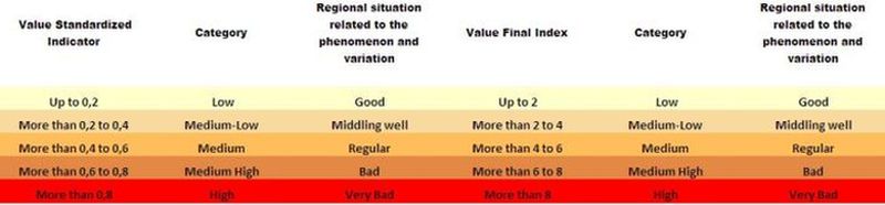
The result of the values obtained for the standard indicators in the year in each dimension is classified into five categories on a scale of increasing intensity of red, interpreted as follows:
(i) when the presence of the phenomenon in the region in the year is up to 0.2, the standard indicator will be considered “low” and so its performance will be “good,” receiving a less intense color on the scale;
(ii) when the presence of the phenomenon is over 0.2 to 0.4 in standard indicator, it will be considered “medium low” and thus its performance will be “good-middling,” receiving a more intense color in relation to the previous classification;
(iii) when the presence of the phenomenon is more than 0.4 to 0.6 in the standard indicator, it will be considered “medium” and thus its performance will be “regular,” receiving a more intense color compared the previous classification;
(iv) when the presence of the phenomenon is over 0.6 to 0.8 in standard indicator, it will be considered “medium high” and thus its performance will be “bad,” receiving a more intense color in relation to the previous classification, and finally;
(v) when the presence of the phenomenon is more than 0.8 to 1.0 standard indicator, will be considered “high” and, consequently, its performance will be “very bad,” getting the most intense color on the red scale, representing the worst possible situation in the evaluation model.
In the case of the standardized indicator for variations in gross indicators, the color scale used is brown, and follows the same logic. Therefore, the categories are produced to complement each other. So, in the matrix of signals, each region is also represented by a color in the Final Index.
Figure 2 below presents the reading model of the standard indicators and final indexes.
The outcome analysis is evidenced by maps, charts and tables that summarize the evaluation results. Moreover, it presents, for the analysis of each indicator panel, scatter charts, which are used to represent both the values in two dimensions (internal and external) of the evaluation. Then there is an abstraction in Figure 3, the scatter chart, in which there is no data to show the essential information for analysis and reading.
Figure 3 General model of the scatter chart of the indicators.
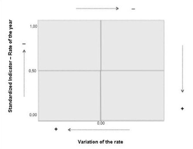
Figures 3 and 4 show the general and reading models, respectively, of the scatter charts of the indicators.
In the y-axis shows the standardized rates, ranging from 0 to 1, of the selected region for study in the year 2010. The x-axis presents the relative variation of gross indicator between 2009 and 2010.
Reading the Y axis, of standard indicator in the year, the closer the region meets the value of one (1), the higher will be the level of phenomenon occurrence in the region (e.g., higher rates of homicide, robberies, etc.). Conversely, the closer the region meets the value of zero (0), the lower the level of phenomenon occurence in the region will be.
The dispersion chart should be read as follows, as shown in the figure:
Figure 4 Model reading of the scatter chart of indicators.
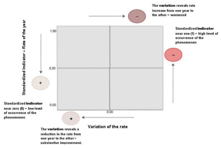
Reading thexX-axis, a region disposed to the right of zero (0), i.e., relative variation of the gross indicator larger than zero (0), showed a poor performance in the previous year. A region disposed to the left of zero (0), i.e., the relative change of the gross indicator smaller than zero (0), improved its performance over the previous year.
Finally, the region which is exactly the value of zero (0) remained stable in the examined indicator between two periods of time.
(* 1) For a description of statistical procedures of standardization of indicators and values for the composition of the synthetic indexes, see the Methodological Annex